Oct 16, 2023
WGSA2 workflow - a tutorial
- Angelina Angelova1,
- Duc Doan1,
- Poorani Subramanian1,
- Mariam Quiñones1,
- Michael Dolan1,
- Darrell E. Hurt1
- 1Bioinformatics and Computational Biosciences Branch, Office of Cyber Infrastructure and Computational Biology, National Institute of Allergy and Infectious Diseases, National Institutes of Health


External link: https://nephele.niaid.nih.gov/
Protocol Citation: Angelina Angelova, Duc Doan, Poorani Subramanian, Mariam Quiñones, Michael Dolan, Darrell E. Hurt 2023. WGSA2 workflow - a tutorial. protocols.io https://dx.doi.org/10.17504/protocols.io.n92ldm98xl5b/v1
Manuscript citation:
Weber N., et al. (2018) Nephele: a cloud platform for simplified, standardized and reproducible microbiome data analysis. Bioinformatics, 34(8): 1411–1413. https://doi.org/10.1093/bioinformatics/btx617
License: This is an open access protocol distributed under the terms of the Creative Commons Attribution License, which permits unrestricted use, distribution, and reproduction in any medium, provided the original author and source are credited
Protocol status: Working
We use this protocol and it's working
Created: July 11, 2023
Last Modified: October 16, 2023
Protocol Integer ID: 84859
Keywords: metagenomic analysis, metagenomics, shotgun, microbiome analysis, assembly, analytical tools, Nephele, WGS, read metagenomic dataset, metagenomics data, metagenomic datasets for deeper exploration, metagenomic short read, metagenomic, shotgun metagenomic short read, free whole metagenome sequencing assembly, computational void in metagenomic, microbiome analysis platform, based microbiome analysis platform, bioinformatics processing, microbiome, complex microbial community, processing raw read, efficient acquisition of biological detail, processing of shotgun dataset, taxonomic annotation, steps of the wgsa2 workflow, shotgun dataset, powerful computational tool, nephele2 team at the national institute, kegg tool, online tool, taxonomic, profiling strategy, extraction of taxonomic, customizations of profiling strategy, wgsa2 workflow, online pipeline, raw read, metacyc, existing tool, tool, blastp, metaphlan, computational resource, wgsa2, development of powerful computational tool
Funders Acknowledgements:
NIH/NIAID
Grant ID: HHSN316201300006W/75N93022F00001
Abstract
The exploration of the microbiome has gained significant attention, leading to the development of powerful computational tools and online pipelines. These tools relieve researchers from the burdensome task of bioinformatics processing for their metagenomics data. Some existing tools (e.g. MetaPhlAn) enable the extraction of taxonomic and functional information directly from shotgun metagenomic short reads. However, more comprehensive analyses rely on tools that often require longer contiguous sequences (e.g. KEGG tools, BLASTp). Unfortunately, there is a scarcity of online tools that provide researchers with computational resources and a command line-free experience to assemble short-read metagenomic datasets for deeper exploration.
To address this computational gap, our Nephele2 team at the National Institute for Allergies and Infectious Diseases (NIAID) designed, developed, and integrated a command line-free Whole Metagenome Sequencing Assembly-based pipeline called WGSA2, into our cloud-based microbiome analysis platform, [Nephele](https://nephele.niaid.nih.gov/). WGSA2 facilitates the processing of shotgun datasets derived from complex microbial communities and diverse habitats, including both host-associated and environmental samples. This pipeline starts by processing raw reads and proceeds to perform functional and taxonomic annotations, to bin the assemblies and to generate graphics to summarize various tabular outputs.
The pipeline offers a user-friendly experience that omits computational demands and expertise. It allows for customizations of profiling strategies and selection of databases (e.g. RefSeq, MGBC, KEGG, MetaCyc). It enables efficient acquisition of biological detail and grants users with easy access to assembly-based sequences and analysis of their datasets. Overall, WGSA2 fills a computational void in metagenomics, enhances accessibility and comprehension of the data, and paves the way for deeper exploration of the microbiome.
This protocol goes through the steps of the WGSA2 workflow, explaining the tools and processing applied in each step.
WGSA2 workflow


Guidelines
This is a tutorial on the usage, processing steps and result interpretation of WGSA2 pipeline hosted on cloud-based microbial analysis platform Nephele (https://nephele.niaid.nih.gov/).
Materials
- Visit Nephele online at https://nephele.niaid.nih.gov/
- Globus endpoint for shotgun metagenomic dataset, shared with Nephele
- Nephele WGSA2-formatted metadata file of your dataset
Troubleshooting
Before start
1) Set up a Globus endpoint for your dataset (if needed). See details here: https://nephele.niaid.nih.gov/using_globus/
2) Download Nephele metadata template for WGSA2 and fill it out. The template is available in the Materials.
Start WGSA2 job
Front page of Nephele Web Platform
Select the "Analyze" tab and proceed to select the WGSA2.2 pipeline.
We will start a WGSA2 job by following simple steps, described below
The "Analyze" tab
Note
We strongly recommend that you first run the Pre-processing (QA) pipeline, and choose to trim and filter reads. This is to ensure only the best quality reads are being used for WGSA2 processing.
You can read more about the QA pipeline from its details page (documentation). An example/template mapping file specific for this QA pipeline can be downloaded here. To download a mapping file for the QA pipeline, use this:  QC_pipeline_template_paired_end_N2.xlsx
Pre-processing tab
Run the "WGSA2" pipeline by clicking the "Start job" button
To initiate a job with WGSA2, click on the "Start job" button. This will take you through the subsequent steps of submitting a job
Selecting the WGSA2 pipeline
Note
You can learn more about this pipeline, its tools, methods and workflow by clicking the 'Learn more' button, or go to https://nephele.niaid.nih.gov/details_wgsa/
General submission tasks (data upload)
More detail about these steps, including how to upload data, can be found in the section "How to submit a job".
Make an account and sign in
In order to run any job in Nephele, you need to make an account using some basic information (<2 min) and log in.
Making an account with Nephele is easy! All you need is an email and a trusty password. The account is free as well as running all the available workflows.
Upload sequence data
Nephele provides multiple ways for data upload including FTP, direct upload and via Globus endpoint. More about how to upload data can be found in the section "How to submit a job".
- The input sequences must be paired-end (PE), whole metagenome shotgun reads (not merged) in FASTQ format.
- No special characters in sequence file names.
- Dataset size should not exceed the 150Gb size limit (gzipped)
- Both zipped (.gz) and unzipped FASTQ files are accepted (.fastq.gz & .fastq)
Note
Due to the huge resource and time requirements of WGSA2, which grows with dataset size, the entire submitted dataset must not exceed 150Gb gzipped. In the rare cases your dataset might exceed this size, please consider splitting it into separate submissions.
Upload metadata
The metadata table will be used by the WGSA2 pipeline to locate and identify your files, associate them with sample names and group them appropriately for the community exploration at the last steps of the pipeline.
This is a tab-delimited file containing information about submitted samples (sample names), the names of their respective FASTQ files, and a simple grouping column (called "TreatmentGroup") that provides grouping information for dataset stats and visualization steps. It is advised such a file is prepared before submission. The template can be downloaded here. Mapping file can be an .xlsx file or a simple .txt file with the following format:
Metadata file format
For your convenience, an example / template metadata file, specific for WGSA2, is attached below.
Note
It is a good rule of thumb to have your metadata file filled out and ready to upload at this step of the job submission. However, it is not a problem if you need to download and fill out the template during submission. You will not be logged out from our system or lose your progress within the submission process, for a few hours.
Main pipeline info
Once your data and metadata are uploaded, the Nephele job submission system will take you to a "Pipeline Selection" screen that allows to you familiarize yourself with the main steps of processing that WGSA2 will go through. This screen is primarily informational and mostly makes you aware that certain processing steps will always happen while others are conditional or optional to datasets (with 2+ samples or user elections). Read through and hit "select".
Pipeline main steps info
Selecting WGSA2 job settings (WGSA2 job options menu)
In this menu, you get to customize the settings of WGSA2 based on your processing needs for your dataset.
WGSA2 job customization options
Apart from the basic Job Name (a brief description of your job for your ease of recognition), these settings include additional trimming and filtering, choice of databases for decontamination, taxonomic classification and metabolic pathways hierarchy. Users may also select WGSA2 to perform additional steps of analysis such as AMR finding, gene-based taxonomic classification, MAGs formation, and more.
Note
The default parameters of WGSA2 are a great starting point for any metagenomic dataset! You may choose to run your first job on any dataset with the pre-set default parameters, and the results will provide you with enough information to familiarize yourself with your dataset's communities and pipeline outputs.
Once you understand the workflow, parameters, and output of the pipeline, you may customize the jobs for any dataset at will.
In the next sections of this protocol, we will be describing what each step of the pipeline's workflow does, and how the customization options from this menu affect the pipeline's behavior and output.
We hope that through those instructions, you will gain the understanding needed to independently choose the best options for any of your datasets and research goals.
Submit job
For now, let us leave the dataset to the default settings (as is) and click 'Submit'.
Your job with WGSA2 will then start, and you will be provided with a job ID. This job ID is important for customer support in case of problems, as well as keeping track of your job status. An email will also be sent to you upon job start and job completion. This email will include the job ID, job details and other job information.
You can have multiple jobs submitted and running at once.
Upon completion of the pipeline, you will be able to view some results directly in your browser. All detailed results and outputs will be provided as downloadable files.
Note
WGSA2 is a completely command line free & automated pipeline. Beyond submitting a job, you will not need to do anything to produce the pipeline results.
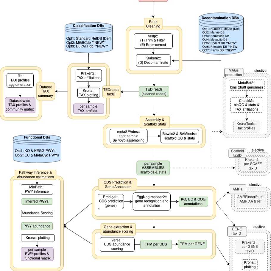
WGSA2 processing: 1 - TEDing module (pre-assembly processing)
30m
(T) Trimming & filtering of raw reads
Note
Note: This step is not as thorough as the recommended pre-processing performed by our QC pipeline and therefore should not be considered as its replacement. If you have run your dataset through the QC pipeline, feel free to leave this option unselected.
In this quick trim and filtering step, WGSA2 verifies that the reads from the submitted dataset have met the minimal quality and length standards required for assembly.
However, if the user has selected customizations through the "Additional trim & filter" option in the Job options menu (see step 6 of this protocol), then those more stringent parameters will be applied.
Additional trim & filter
Note
If you choose to select the additional trim and filter checkbox from the WGSA2 options menu (see step 6 of this protocol), a few more options will appear where you can provide more detail for the trimming & filtering parameters of your choice.
5m
(E) Error-correction
PE sequences are merged, and sequencing errors are corrected within the PE overlapping regions. This process is specifically designed to improve assembly efficiency and success.
This process is mandatory for the pipeline and undergoes no customization (see step 5, Pipeline selection section)
5m
(D) Decontamination
In the pre-assembly processing, the dataset undergoes a thorough cleaning process to remove host DNA and non-informative elements, such as homopolymeric or simple sequence repeats. This is achieved by utilizing a Host Decontamination database, containing a curated collection of thematically related host organism genomes.
The decontamination process is crucial for reducing the dataset size, by excluding biologically irrelevant data (non-informative host DNA, junk and repeat sequences). Thus the assembly quality of each sample is significantly improved.
The Host Decontamination database used in this processing step, is user-electable in the Job options menu (see step 6 of this protocol). By default, WGSA2 will decontaminate any dataset against the Human & Mouse DB, however you may elect (from the drop-down menu of the Job Options) a more appropriate decontamination database for your submitted dataset, depending on the host organism or environment from which your dataset's microbial community is collected.
Host Decontamination DB choices
All decontamination databases of WGSA2 are custom curated based on a theme of host organisms or environments that a microbial community might be sourced from.
The user choices for Host Decontamination DBs are:
- Human & Mouse Host DB (includes human + mouse host genomes)[default DB for quickest removal of most common host contaminants]
- Marine Hosts DB (includes human + 18 common marine host organism genomes)
- Mosquito Hosts DB (includes human + 2 common mosquito species genomes)
- Nematode Hosts DB (includes human + 15 common nematode host organism genomes)
- Rodent Hosts DB (includes human + 5 common rodent host organisms)
- Primates Hosts DB (includes human + 9 common primate host organisms)
- Plant Hosts DB (includes human + >110 common plant host organisms)
Please see WGSA2's documentation page for more detail on the specific genomes and assembly versions each database contains.
15m
TEDing module outputFrom 5 to 14 steps
The TEDing module will output the same TED reads:
These are the cleaned sequences of your dataset that have undergone
1) Trimming & filtering,
2) Error-correction, and
3) Decontamination from host genomic and repeat sequences
Upon pipeline completion, you may download the resulting output folder from your WGSA2 job, and find these
TED reads in subfolder named "TEDreads"
The TEDreads folder will contain per-sample logs and reports from the TEDing steps ( e.g. _fastplog.html ,
_decontamLOG.txt & more), where you can find information about the trimming success & host
contamination levels removed from each sample.
Content of TEDreads/Samp1_decontamLOG.txt
WGSA2 processing: 2 - TAX profiling module
30m
Taxonomic profiling
Performed with Kraken 2
By default, WGSA2 generates taxonomic profiles from the TEDreads of every sample individually, utilizing the Kraken2 tool. This highly accurate and computationally efficient method for taxonomic identification relies on a comprehensive database of k-mers derived from entire genomes of known organisms. This enables accurate taxonomic assignments for both coding and non-coding sequences, contained within the TEDreads.
For this processing step, the taxonomic classification DB is also user-electable. The applied default is a Kraken2 version of NCBI's RefSeq DB (Kraken2 Standard Reference Genomes DB; kr2_REFdb). However, depending on interest and dataset source, user may choose one of a few other options: The Mouse Gastrointestinal Gut Catalogue DB (MGBCdb), containing >26.6K prokaryotic organisms characteristic for mouse gut microbiomes (both reference and non-reference organisms), and the Eukaryotic Pathogens DB (EuPATHdb), containing genomes of known eukaryotic pathogens.
For more information about the available classification DBs, please, refer to WGSA2 documentation page.
To have WGSA2 perform TAX classification based on a different DB, other than the default, the user may elect a taxonomic classification DB in the Job options menu (see step 6 of this protocol) upon job submission.
Taxonomic classification DB
30m
TAX profile visualizations
Performed with Krona Tools
In this processing step, the resulting taxonomic profiles (from the previous step) are re-formatted and visualized using Krona tools on a per-sample basis. The resulting plots are in HTML format and present the community's taxonomic composition in a circular interactive plot produced per sample. With the latest WGSA2 pipeline update, the highest taxonomic level is presented in the taxonomic ID (UUID or TAXid) for each detected organism.
Example Krona taxonomic profile plot (per sample)
Note
Since the MGBCdb include non-reference organisms and taxonomically undefined (yet) genomes, its taxonomic IDs do not correspond to NCBI's UUIDs.
2m
Files associated with Krona visualizationsFrom 3 to 12 steps
The output from this module can be found in the WGSA2 results folder:
TAXprofiles > readsTAX_{DBname}/, where the {DBname} suffix will be
naming the TAX classification DB elected by user.
The outputs of the Kraken2 step are text format samples, contained within the
> reports/ folder . These text files are used for community profiles visualizations,
as well as in the subsequently produced dataset-wide community matrix table,
which is the foundation of microbial community analysis studies.
The krona re-formatted Kraken2 reports (produced from the previous step) can be found in
the > bin/ foler. Those are used by KronaTools to produce the interactive HTML report
TAXprofiles > readsTAX_{DBname} > TAXplots_readsTAX_<DBname>.html
WGSA2 processing: 3 - Assembly module
10h
Assembly
In this step, a de novo assembly of the TED reads is performed for each sample independently. This produces long contiguous sequences (contigs), that are then arranged, oriented, and connected (with Ns), based on PE data of the incorporated reads until scaffolds of contigs are achieved. As metagenomic datasets are composed of numerous genomes, the produced assemblies are composed of numerous long (and short) scaffolds, each representing a genomic loci of a contained organism.
Note
This is a rather time and resource consuming step and tends to take even longer for large datasets containing complex communities! Please be patient with the WGSA2 processing.
4h 30m
Assembly processing - Read mapping (read alignments)
In this step the TED reads are again used to align to the corresponding sample’s scaffolds (a process called ‘mapping’). The alignment of the reads is also QC’d and cleaned (de-replicated, mate pairs are fixed, etc.) to ensure each pair of reads maps best and only once to the produced assembly.
Note
This is one of the most time and resource consuming stages of the pipeline and depending on sample size may take longer than a few hours per sample. Parallelization is used to achieve assembly of multiple samples simultaneously (however, patience is still required). Pipeline failures in this processing stage suggests problematic sample depths or read quality.
4h 30m
Assembly processing - Abundance scoring
The aligned reads are evaluated (GC content, plus/minus strand alignments) and enumerated. Abundance scores are produced per scaffold per sample (scaffold length, depths, coverage, reads per million (RPM), etc.), and other statistics are collected. This information is used for downstream abundance assessments, as well as every other downstream processing step of the pipeline.
10m
Output of processed assemblyFrom 3 to 9 steps
For each assembled sample an individual folder is produced:
asmbMetaSpades > {SampleName}_asmb/
This collects only that sample's information, including the assembly's FASTA file,
assembly stats, alignments and all other files related to the processed assembly.
All files produced from the assembly (step 13) and assembly processing steps (steps 14-15)
carry the {final.assembly} prefix and are the main files used for all
downstream processing. These include:
- final.assembly.fasta (the FASTA representation of the assembled sample)
- final.assembly_stats.txt (statistical information about the assembled sample (e.g. N50)
- final.assembly_scaffCoverage.txt (scaffold abundance, coverage, read counts, length and
other per-scaffold in {SampleName} related information
- final.assembly.bam (processed read alignment file) [can be used if user wishes to extract
specific short reads aligned to a genomic locus of choice (e.g. gene)]
- contigs.fasta (a contig-based representation of the assembled sample)
Note:
Sub-folders are also present within this main assembly folder. Those are produced from
other, subsequent steps of the WGSA2 pipeline and may vary based on user options elected.
The content of such sub-folder will be described in the corresponding sections.
WGSA2 processing: 4 - Gene discovery module
6h
Gene prediction
Performed with Prodigal
The tool scans through scaffold sequence in each sample and predicts potential partial or full-length continuous coding regions (features, genes) that commonly occur in prokaryotes, and unicellular eukaryotes.
30m
Gene abundance scoring
Gene abundance scores are computed by enumerating the number of reads aligned to the gene coordinates of the scaffold.
Reads per Million (RPM) mapped reads and transcripts per million (TPM) values are calculated based on per transcript instance in each scaffold in each sample and produce the abundance scores of each gene.
In WGSA2 pipeline, the notation 'iTPM' is used to denote conventional TPM scores. This is to distinguish from another statistic of the pipeline 'geneTPM' which represents calculated average abundance score (TPM) for each unique annotation within sample. A geneTPM abundance matrix is also provided with WGSA2.
15m
Gene prediction & abundance scoring resultFrom 1 to 7 steps
Expected output is contained within each sample's assembly folder at:
asmbMetaSpades > {SampleName}_asmb > genes/ folder.
This includes files with the PREDgenes prefix, containing the predicted gene's NT and AA sequence information
(PREDgenes.fna and PREDgenes.faa) as well as a gene annotation file (PREDgene.gff). These files can be used
by the user for custom gene annotation (e.g. the KEGG's GhostKoala tool) or identifying the location coordinates
of each predicted feature.
The outputs also contain summary statistics information such as gene scoring stats (PREDgenes_stats.txt) and
gene abundance information (PREDgenes_ABUN.txt), such as gene length, aligned reads, coverage, RPK of gene
and gene's iTPK (the TPM for that particular instance of the gene).
The predicted features are compared to a database of known genes (EggNOG-v5) and upon sufficient homology the gene annotation is transferred to the feature. Gene annotations obtained are based on KO, EC and COG annotation systems.
4h
Gene annotations6 steps
Gene annotations are outputted in the folder:
asmbMetaSpades > {SampleName}_asmb > genes > annotations/.
The content includes the annotations ({annots} prefix) produced by the EggNOG-mapper2, as well as
the NT and AA files based on the KEGG (annots.ko.{faa, fna, txt}) and the EC annotations
(annots.ec.{faa, fna, txt}).
Important summary and abundance scoring files from the annotated output are presented in the
ANNOTgenes_ABUNDtab.{ko,ec}.txt files (including the iTPM for each instance of the annotated gene).
With the latest WGSA2 update, the pipeline now also outputs a per unique gene annotation summary
files {SampleName}_geneTPM.{ko, ec}.txt, which contains the average TPM per unique annotation
(geneTPM) as well as the gene's short and long names. These are also gathered from each sample and
stored at PWYprofiles/<PWYdb_name>/genebin/ for downstream utilization (e.g. data collation).
WGSA2 processing: 5 - Pathway profiling module
30m
Pathway (PWY) inference
Performed with MinPath
The produced gene annotations (KO or EC) are mapped against a user-elected database of cellular pathways (KEGG or MetaCyc). A parsimony approach is then used to reconstruct the minimal set of pathways (from the selected DB) that can be described by the annotations (query of genes) within each sample (MinPath).
The default WGSA2 database for PWY inference is the KEGG db, along with the KO annotations produced in each sample. Users may opt for a different approach: to use the EC annotations of the samples to map against the MetaCyc db of pathways (instead of KEGG), which provides a different metabolic PWY classification system and will therefore produce a slightly different metabolic representation for each sample. The DB of choice is to be elected based on your convenience and familiarity. Although the results may slightly differ, there is no known incorrect option.
PWY DB election
15m
PWY abundance estimation
The abundance of each pathway is then calculated by averaging the TPM values from each instance of gene, within each inferred pathway.
10m
PWY profile visualizations
Performed by Krona Tools
The metabolic characterization for each sample (representing the functional profile) are summarized for each sample in an interactive HTML report.
PWY krona plot
5m
PWY inference & profiling3 steps
The PWY inference and abundance estimation text reports are outputted in folder
asmbMetaSpades/{SampleName}_asmb/genes/pathways/.
Among these files is a text report of the final functional profile from each sample ({SampleName}_4krona.txt).
This file is collected from each sample and gathered into a pwy_bin/ folder at PWYprofiles/<PWYdb_name>/pwy_bin/
for downstream utilization (e.g. KronaTools visualizations, data collations, etc)
To obtain a visual representation of these functional profiles, KronaTools is again used. The functional profile HTML
interactive report is presented in PWYprofiles/<PWYdb_name>/PWYplots_<PWYdb_prefix>.html, where
<PWYdb_prefix> is either ko2gg or ec2mc, depending on user election if functional database.
WGSA2 processing: 6 - Dataset summary module
20m
Data collation
The steps in this module are among the most important ones for the summary characterizations of any dataset. Since the pipeline has already created per-sample individualized profiles and summaries, this module is conditional to datasets with multiple samples (best if >2 samples).
In this module, the feature characterizations and abundance information from each individual sample are collected and summarized (collated) into a dataset-wide abundance matrix. This matrix is a non-redundant feature (TAX, PWY or GENE) representation of each sample's composition (abundance matrix).
Note
The abundance matrix is a table that contains the feature identity (taxonomic or functional) and abundance information for each sample within a dataset. It is the abundance matrix that is the fundamental part of any downstream community-based microbial exploration.
Example feature abundance table
15m
Convert to biom format
Performed by biom-format
The taxonomic and functional abundance matrices are further formatted into biom files that include the user metadata. These biom files can be conveniently uploaded into [MicrobiomeDB] or customized as needed for other user-specific purposes.
5m
Abundance matrixes1 step
All the most important taxonomic and functional analysis compositional abundance matrices created
during the pipeline run, can be found within the merged_tables/ folders within the corresponding
TAXprofiles or PWYprofiles/ folders.
These compositional tables include:
- Taxonomic compositional matrix for dataset - the taxonomic information and abundance from each
sample, collated into one non-redundant matrix. This is used for any taxonomic microbiome
analysis and statistical comparison between communities. Stored in
TAXprofiles/readsTAX_<DBname>/merged_tables/merged_Counts+TAX.txt
- Genetic compositional matrix for dataset - the gene information and abundance from each sample
collated into one non-redundant matrix. This is used for any gene-focused microbiome explorations.
Stored in PWYprofiles/<PWYdb_name>/merged_tables/merged_geneTPMtable.txt
- Pathway compositional matrix for dataset - the functional (inferred pathway) information and
abundance from each sample, collated into 1 non-redundant matrix. This is used for any functional
analyses of communities and statistical comparisons between them. Stored in
PWYprofiles/<DBname>PWYs.MP/merged_tables/merged_Counts+PWY.txt
All files in these folders have a generally similar structure. They represent an abundance matrix for
the dataset, inclusive of all the samples and various features (TAX or PWYs or GENEs). This
information however is presented in different ways:
1) the per-sample counts alone (merged_Counts.txt)
2) the features identities alone (merged_{TAX, PWY}.txt)
3) the per-sample counts with the features table adjoined, in various combinations: each rank/level as
separate columns (merged_Counts+{TAX, PWY}.txt), or concatenated together as lineage within 1
column (e.g. merged_Counts+Lineage.txt), or both (merged_Counts+TAX+Lineage.txt).
4) the per-sample abundance table (merged_Counts+Lineage.txt), presented as a json biom file
(merged_Counts+Llineage_json.biom).
These files present the same information but separated by format for convenient utilization in
downstream analytical tools.
Exploratory visualizations and statistics
The steps in this module are conditional to datasets containing multiple samples (best if >3 samples), as they require statistical calculations and summary visualizations.
The obtained TAX and PWY abundance matrices, are used to produce community characterizing visualization plots (e.g. alpha and beta diversity plots, abundance profile heat-maps etc.). These are especially useful for quick familiarization with the composition of the samples in your dataset and understanding some of the community relations.
10m
Protocol references
References
- Shifu Chen, Yanqing Zhou, Yaru Chen, Jia Gu, fastp: an ultra-fast all-in-one FASTQ preprocessor, Bioinformatics, Volume 34, Issue 17, 01 September 2018, Pages i884–i890, https://doi.org/10.1093/bioinformatics/bty560
- Bankevich et al. SPAdes: A New Genome Assembly Algorithm and Its Applications to Single-Cell Sequencing. J Comput Biol. 2012 May; 19(5): 455–477.doi: 10.1089/cmb.2012.0021
- Langmead, B., Trapnell, C., Pop, M. et al. Ultrafast and memory-efficient alignment of short DNA sequences to the human genome. Genome Biol, (2009). https://doi.org/10.1186/gb-2009-10-3-r25
- Li H, Handsaker B, Wysoker A, Fennell T, Ruan J, Homer N, Marth G, Abecasis G, Durbin R; 1000 Genome Project Data Processing Subgroup. The Sequence Alignment/Map format and SAMtools. Bioinformatics. 2009 Aug 15;25(16):2078-9. doi: 10.1093/bioinformatics/btp352. Epub 2009 Jun 8. PMID: 19505943; PMCID: PMC2723002.
- Kang, Dongwan D et al. MetaBAT 2: an adaptive binning algorithm for robust and efficient genome reconstruction from metagenome assemblies, PeerJ. 2019, doi:10.7717/peerj.7359
- Cantalapiedra Carlos P., Hernandez-Plaza Ana, Letunic Ivica, Bork Peer, Huerta-Cepas Jaime. eggNOG-mapper v2: functional annotation, orthology assignments, and domain prediction at the metagenomic scale. biorxiv. (2021) doi: https://doi.org/10.1101/2021.06.03.446934
- Hyatt, Doug et al., Prodigal: prokaryotic gene recognition and translation initiation site identification., BMC bioinformatics vol. 11 119. 8 Mar. 2010, doi:10.1186/1471-2105-11-119
- Parks, Donovan H et al., CheckM: assessing the quality of microbial genomes recovered from isolates, single cells, and metagenomes., Genome research vol. 25,7 (2015): 1043-55. doi:10.1101/gr.18607214
- Ondov, B.D., Bergman, N.H. Phillippy, A.M. Interactive metagenomic visualization in a Web browser. BMC Bioinformatics, 385 (2011). https://doi.org/10.1186/1471-2105-12-385
- Ye Y, Doak TG (2009) A Parsimony Approach to Biological Pathway Reconstruction/Inference for Genomes and Metagenomes. PLOS Computational Biology 5(8): e1000465. https://doi.org/10.1371/journal.pcbi.1000465
- Caspi et al 2020, The MetaCyc database of metabolic pathways and enzymes - a 2019 update, Nucleic Acids Research 48(D1):D445-D453
- Zhu, Q., Fisher, S.A., Shallcross, J., Kim, J. (Preprint). VERSE: a versatile and efficient RNA-Seq read counting tool. bioRxiv 053306. doi: http://dx.doi.org/10.1101/053306
- Carlos P. Cantalapiedra, Ana Hernandez-Plaza, Ivica Letunic, Peer Bork, and Jaime Huerta-Cepas., eggNOG-mapper v2: functional annotation, orthology assignments, and domain prediction at the metagenomic scale. 2021, Molecular Biology and Evolution, https://doi.org/10.1093/molbev/msab293
- Minoru Kanehisa, Yoko Sato, Masayuki Kawashima, Miho Furumichi, Mao Tanabe, KEGG as a reference resource for gene and protein annotation, Nucleic Acids Research, 2016, https://doi.org/10.1093/nar/gkv1070
- Wood, D.E., Lu, J. & Langmead, B. Improved metagenomic analysis with Kraken 2. Genome Biol, 2019. https://doi.org/10.1186/s13059-019-1891-0
- R Core Team (2021). R: A language and environment for statistical computing. R Foundation for Statistical Computing, Vienna, Austria. URL