Jan 20, 2023
Version 2
Topographical mapping of sympathetic postganglionic innervation of mouse heart V.2
- Ariege Bizanti1,
- Yuanyuan Zhang1,
- Kohlton Bendowski1,
- Jin Chen1,
- Mahyar Osanlouy2,
- Maci Heal3,
- Zixi Jack Cheng1
- 1University of Central Florida;
- 2Auckland Bioengineering Institute;
- 3MBF Bioscience
- SPARCTech. support email: [email protected]


Protocol Citation: Ariege Bizanti, Yuanyuan Zhang, Kohlton Bendowski, Jin Chen, Mahyar Osanlouy, Maci Heal, Zixi Jack Cheng 2023. Topographical mapping of sympathetic postganglionic innervation of mouse heart. protocols.io https://dx.doi.org/10.17504/protocols.io.n92ldzbmxv5b/v2Version created by Ariege Bizanti
License: This is an open access protocol distributed under the terms of the Creative Commons Attribution License, which permits unrestricted use, distribution, and reproduction in any medium, provided the original author and source are credited
Protocol status: Working
We use this protocol and it's working
Created: January 19, 2023
Last Modified: January 20, 2023
Protocol Integer ID: 75600
Keywords: topographical mapping of sympathetic postganglionic innervation, sympathetic postganglionic axon, immune reactive sympathetic postganglionic axon, sympathetic postganglionic innervation, terminals in the mouse heart, topographical organization of tyrosine, mouse heart, topographical mapping, mouse heart this protocol, topographical organization, microscopy, heart
Funders Acknowledgements:
HEAL/SPARC
Grant ID: NIH U01 NS113867-01
NIH R15
Grant ID: NIH R15HL137143-01A1
Abstract
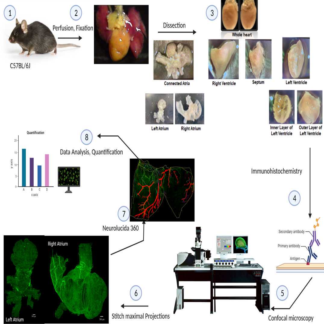
This protocol describes the process of mapping the topographical organization of tyrosine hydroxylase immune reactive sympathetic postganglionic axons and terminals in the mouse heart. Hearts were removed and separated as whole mounts, then scanned using confocal or zeiss microscopy
Workflow
Animals
Male C57BL/6J mice (Jackson laboratory), n=6 were used. Animals were kept in the animal room with dark/light cycle set to 12/12 hours and water and food were supplied ad libitum. All procedures were carried out under the ethical guidelines of University of Central Florida and approved by the Animal Care and Use Committee of University of Central Florida.
Perfusion and tissue preparation
Animals were were anesthetized with sodium pentobarbital injection (i.p., 100 μg/g). As the animals did not have hind paw pinch withdraw reflex, the chest cavity was opened and heparin (0.2ml; 1,000 units/ml) was injected into the left ventricle, followed by transcardial perfusion. Mice were perfused with at least 150 mL 40 °C phosphate-buffered saline (0.1 M PBS, pH = 7.4) at a rate of approximately 40 ml/min, effectively draining the animal of blood via a blunt 18-ga needle inserted to the left ventricle , and blood was drained by cutting the inferior vena cava. The perfusion solution was switched to 150 mL ice cold Zamboni’s fixative (15% picric acid, 2% paraformaldehyde in PBS, pH = 7.4) to fix the tissue. During the entire procedure, extreme care was taken to ensure that no part of the heart or intestine became dry in an effort to minimize autofluorescence during later examination. After the perfusion, the mice heart was removed and post fixed overnight.
Immunohistochemistry
All IHC steps were performed using a 24-well plate on a shaker at room temperature (~24 °C) in dark environment, with each piece of tissue immersed in 0.5 ml of reaction liquid in its own well. The IHC steps include washes, blocking, primary antibody, secondary antibody, and were carried out in different wells. Samples were washed 6x5 minutes in 0.1 M PBS (pH = 7.4) and immersed in blocking solution (0.1 M PBS containing 2% bovine serum albumin, 10% normal donkey serum, 2% Triton X-100, and 0.08% sodium azide) for 48 hr.
Primary antibodies (12 μl/ml each , see Table 1 for details) were added to primary solution (2% bovine serum albumin, 4% of normal goat serum, 4% normal donkey serum, .08% Triton X-100, .08% NaN3 in .1 M PBS, pH=7.4) and administered for 48 hr. Unbound primary antibodies were removed from tissues by six 5 min washes in PBST (0.3% Triton X-100 in 0.1 M PBS, pH=7.4).
Secondary antibodies (12μl/ml each, see Table 1 for details) were then applied for 24 hr. Unbound secondary antibodies were removed from tissues by six 5 min washes in PBS.
| A | B | C | D | E | F | G | |
| Antibody | Concentration | Host | Company | Cat # | Emission | RRID | |
| Anti-TH | 1:100 | Rabbit | Pel-Freez | P40101-0 | n/a | RRID:AB_461064 | |
| Anti-TH | 1:100 | Sheep | Millipore | AB 1542 | n/a | RRID:AB_90755 | |
| Donkey Anti-Rabbit | 1:50 | Donkey | Invitrogen | A21206 | 488 | RRID:AB_2535792 | |
| Donkey anti-sheep | 1:50 | Donkey | Invitrogen | A-11016 | 594 | RRID:AB_2534083 |
Table 1: Antibodies sources and concentration
Tissues were then mounted with their cranial surface (in the case of the atria) or dorsal surface (in the case of the ventricles) down onto positively-charged glass slides, crushed overnight , and air-dried.
Slides were dehydrated by immersing them for 2 minutes in each of 4 ascending concentrations of ethanol (75%, 95%, 100%, 100%), followed by two 10 min washes in 100% xylene. Slides were then coverslipped with DEPEX mounting medium (Electron Microscopy Sciences #13514) and allowed to dry overnight. Care was taken during every step of this procedure to minimize tissue exposure to light and to prevent tissue from becoming dry.
Tissue scanning
The samples were scanned with two microscopes: one is Leica TCS SP5 Confocal Laser Scanning Microscope. Argon-krypton laser was excited at 488 nm and emitted at 500-550 nm to detect TH-IR axons. Image stacks of 1.5-1 μm z-acquisition were saved as .lif and fully projected confocal images were saved as .tif. All image tiles were stitched together using Adobe Photoshop to assemble the montage of the whole heart. Another microscope is ZEISS Axio Imager M2.
Neurolucida 360
Have Neurolucida 360 installed and licensed on your workstation through an MBF Bioscience representative
[https://www.mbfbioscience.com/neurolucida360]
After launching Neurolucida 360, set an API key to your profile to pull the ontology list from SciCrunch to annotate your organ of choice with curated SPARC anatomy terms (you might have to register an account on scricrunch.org in order to obtain an API key).
Image annotation and Nerve tracing Opening and configuring the image file: In the "File" ribbon and under the "Open" menu, select "Image," and select the image file (.jpg or .tif) of interest. A dialog will appear to verify or adjust the XY scaling properties of the image. If the scaling properties are correct and do not need adjustment, click "OK" to load the image.
Contour the sample: To begin contouring or tracing anatomical features, go to the "Trace" ribbon and in the "CONTOURS" submenu, click "Contour selection" to display the list of curated SPARC anatomy terms.
Nerve tracing: To enable neuronal tracing mode, go to the "Trace" ribbon and in the "NEURONS" submenu, click "Axon".
o preserve your progress in annotating and tracing, go to the "File" ribbon and under the tab "Save as," select "Data File" and save your work as an XML document file (.xml). The associated metadata from the initial dialog box will autopopulate when you load the file to resume your work.
Metadata setup: Create a profile for your sample by filling in the subject information of your sample with the species, sample ID, sex, and age on the left side of the dialog. Then specify the species and organ in which you are annotating on the right side of the dialog to access the curated SPARC anatomy terms and click "Begin" when you are done. For the purposes of our tracing, the organ is the "Heart" and the species is "Mus musculus". Manually inputting information about your sample only occurs once when you first create a document to annotate your sample. After you save your work as an .xml file and load it into the program, the metadata dialog will autopopulate and you can resume your work.
More detailed description of Neurolucida 360 use in our lab is explained in a previous protocol
Integrating tracing data into 3D heart Scaffold
Tracing data of sympathetic postganglionic innervation of heart tissue saved as XML will be integrated into 3D heart scaffold