Jul 15, 2020
Version 2
Fitting enzyme kinetics data with Solver V.2
This protocol is a draft, published without a DOI.
- 1James Madison University


Protocol Citation: Nithesh Chandrasekharan, Chris Berndsen 2020. Fitting enzyme kinetics data with Solver. protocols.io https://dx.doi.org/Version created by Chris Berndsen
Manuscript citation:
Kemmer, G., and Keller, S. (2010) Nonlinear least-squares data fitting in Excel spreadsheets. Nat. Protoc. 5, 267–281.
License: This is an open access protocol distributed under the terms of the Creative Commons Attribution License, which permits unrestricted use, distribution, and reproduction in any medium, provided the original author and source are credited
Protocol status: Working
We use this protocol and it's working
Created: July 15, 2020
Last Modified: July 15, 2020
Protocol Integer ID: 39295
Keywords: kinetics, excel, solver, data fitting, fitting enzyme kinetics data with solver reaction kinetic, fitting enzyme kinetics data, enzyme kinetics data, solver reaction kinetic, kinetic value, kinetic values like the vmax, approximate affinity between biomolecule, functions of enzyme, biochemistry, fundamental skill in biochemistry, enzyme, fundamental component of the biochemical characterization, biochemical characterization, students in biochemistry, biomolecule, several substrate concentration, other biomolecule, approximate affinity, km value, work of kemmer,
Abstract
Reaction kinetics are a fundamental component of the biochemical characterization of a biomolecule. The Vmax and the KM values derived from experiments describe how fast a biomolecule catalyzes the reaction and the approximate affinity between biomolecule and substrate. For almost a century, these properties have been used to describe the mechanism and functions of enzyme and other biomolecules. Fitting data to calculate kinetic values like the Vmax and the KM values is a fundamental skill in biochemistry.
This protocol describes fitting data determined at several substrate concentrations to calculate Vmax and KM values using Excel/Google Sheets and the macro with these programs Solver. This protocol is based on the work of Kemmer and Keller.
This protocol is written for students in Biochemistry at James Madison University, however the approach is general enough for any enzyme kinetics data.
Materials
Microsoft Excel or Google Sheets
Kinetics data from at least 5 concentrations of substrate
Where to start
If you have calculated rate data already skip to step 2.3. If you have time course data and need to calculate the rate, start with step 2.
Calculating intial rates
Calculate the initial rate from the slope of the product formed vs. time plot.
Note
It is important to calculate the rate when the plot of product formed vs. time is linear with time. This ensures that the enzyme is in the steady-state. Typically this is in the early part of the reaction before more than 10% of the substrate has been converted to product (see figure). The rate is the slope of the line.
In the steady-state, the concentration of enzyme bound complexes is not changing with time and the enzyme is catalyzing the reaction at the fastest possible rate at that concentration of substrate.
Example of fitting to calculate the initial velocity. Blue points are data. Blank dashed line shows the fitting of the trendline to the portion of the data where it is linear and presumably the reaction is still in the steady-state. The slope of the black dashed line would be the initial velocity or initial rate.
Repeat for each concentration of substrate.
Subtract the rate of the background reaction from each rate.
Note
Background rate is typically from a reaction performed in the absence of enzyme which shows the rate of the reaction in the absence of catalysis.
Record the rate at each concentration of substrate in the table below. Be sure to modify the units to match the units from the experiment. Add rows to the table as needed.
| Concentration of substrate (uM) | Observed Rate (uM/sec) | |
Plotting data to estimate kinetic values
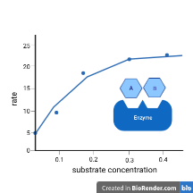
Plot rate (y-axis) vs Substrate concentration (x-axis) and estimate the Vmax and KM values using the plot. Plot the data as a scatter plot (no lines)
Note
The Vmax estimate is the y-value where the graph levels out. The KM is the x-value at 1/2 Vmax.
Record your estimates with units of Vmax and KM in the table below.
| Vmax | |||
| Km |
Fitting data to calculate Vmax and Km
To draw a trendline, you'll need to calculate theoretical values for rates using the estimated Vmax and KM values from 2.1 and the Michaelis-Menten Equation. This is your V Calculated (V calc). This will also help you calculate the correct Vmax and Km values later on.
In Microsoft Excel or Google Sheets, set up a table with headers as shown below:
| Concentration of substrate | Observed rate | Theoretical rate (V Calc) | Squared residual | Variables | Estimates | Units | ||
| Vmax | ||||||||
| Km | ||||||||
| SSR |
Input your data table from step 1.3 into columns A and B.
Input your estimates of Vmax and KM from step 2.1 into the appropriate box in column G
In column C, insert the following code to use the Michaelis-Menten equation to calculate the theoretical rate given the estimates for Vmax and KM.
=($G$2 * A2)/($G$3 + A2)
Note
This code uses the Michaelis-Menten equation
"Drag" the equation down until the theoretical rate has been calculated for all the concentrations of substrate. After this step the table will appear similar to below:
In Column D, insert the following code to calculate the squared residual value.
=(B2-C2)^2
Note
The squared residual will be used to calculate error and refine the estimates of Vmax and KM. It is the squared difference between the real rate and the calculated rate. For a perfect match the squared residual should be zero.
"Drag" the equation down until the squared residual has been calculated for all the concentrations of substrate.
In cell G4, insert the following code to calculate the sum of squared residuals. Replace DXX with D followed by the number of the last substrate concentration (e.g. D10 if there are 9 substrate concentrations).
The resulting number is the sum of squared residuals or SSR.
=sum(D2:DXX)
Use SOLVER to fit the data by changing the Vmax and KM estimates to minimize the sum of squared residuals.
If Solver has not been used before, it may not have been installed as described below. If it has been used before skip to step 6.2.
Note: For some users of Excel, add-ins are disabled, therefore Google Sheets has to be used.
FOR EXCEL USERS:
If Solver has not been installed, it can be added to Excel by going to File -> Options -> Add-ins -> Manage Excel Add-ins -> Solver Add-in
FOR GOOGLE SHEETS USERS:
If Solver has not been installed, it can be added to Sheets by going to Add-ons -> Get Add-ons, and searching for Solver.
Load the Solver window. In Excel, Solver is found in the Data tab. In Sheets, it is found in the Add-ons menu.
The Solver window (example from Excel shown below) has 4 parameters to set:
- Set Objective: $G$4
- To: Min
- By Changing Variable Cells: $G$2, $G$3
- Select a Solving Method: GRG Nonlinear
The Objective and Variable cells can also be selected using the button at the right of the window and using the cursor to click on the appropriate cells.
Solver in Google Sheets
Solver in Excel
Click Solve and wait for the fitting to finish (<10 seconds).
Note
Solver will subsitute in various values for Vmax and KM to reduce the SSR value as much as possible which means that the theoretical values match the experimental values closely. At the end, the values will be changed automatically in the spreadsheet
In Sheets: Solver will run and change the values.
In Excel: A window will pop-up asking to accept the values and display if there were errors. Click OK and the estimated Vmax and KM will be changed to the optimized values.
Record the values Vmax, KM, and SSR below. These Vmax and KM values are accurate compared to your original estimates.
| Vmax | ||
| Km | ||
| SSR |
Visualizing the fit to the data
Add a second set of data to the original plot of observed rate vs. concentration of substrate.
Plot the theoretical (V Calc) rates vs. concentration of substrate.
Click on the newly plotted V Calc data and edit the data set to show only the line.
To show only the line, highlight the Vcalc data by left-clicking on the data and then right clicking to bring up the pop-up menu. Format the data series to add the line.
The plot should look similar to that shown below:
Label the plot axes with appropriate labels and units.
Save your plot as a picture and upload the image.