Jan 31, 2024
Version 2
Characterization of human immune cell subpopulations in cerebrospinal fluid using mass cytometry. V.2
- Gerardina Gallaccio1,
- Meng Wang1,
- Stephan Schlickeiser2,
- Desiree Kunkel3,
- chotima.boettcher 1,
- Camila Fernández-Zapata1
- 1Experimental and Clinical Research Center, a cooperation between the Max Delbrück Center for Molecular Medicine in the Helmholtz Association and Charité-Universitätsmedizin Berlin, Berlin, Germany. Max Delbrück Center for Molecular Medicine in the Helmholtz Association (MDC), Berlin, Germany. Charité-Universitätsmedizin Berlin, corporate member of Freie Universität Berlin and Humboldt-Universität zu Berlin, Berlin, Germany.;
- 2Institute of Medical Immunology, BIH-Center for Regenerative Therapies, Charité-Universitätsmedizin Berlin, and Berlin Institute of Health Berlin, Berlin, Germany.;
- 3Berlin Institute of Health at Charité - Universitätsmedizin Berlin, Flow & Mass Cytometry Core Facility, Berlin, Germany.


Protocol Citation: Gerardina Gallaccio, Meng Wang, Stephan Schlickeiser, Desiree Kunkel, chotima.boettcher , Camila Fernández-Zapata 2024. Characterization of human immune cell subpopulations in cerebrospinal fluid using mass cytometry.. protocols.io https://dx.doi.org/10.17504/protocols.io.36wgqjp4ovk5/v2Version created by Gerardina Gallaccio
Manuscript citation:
License: This is an open access protocol distributed under the terms of the Creative Commons Attribution License, which permits unrestricted use, distribution, and reproduction in any medium, provided the original author and source are credited
Protocol status: Working
We use this protocol and it's working
Created: January 31, 2024
Last Modified: January 31, 2024
Protocol Integer ID: 94450
Keywords: immune profiling, dimensional immune profiling, track disease activity for neuroinflammatory, using cytometry, characterization of human immune cell subpopulation, using mass cytometry, cerebrospinal fluid, cytometry by time, mass cytometry, human immune cell subpopulation, compositional changes of immune cell, cell resolution, immune cell, neuroinflammation, neuroinflammatory, cytof, biomarker, csf of patient, neurodegenerative disease, track disease activity, cell
Abstract
Phenotypic and compositional changes of immune cells in cerebrospinal fluid (CSF) can be used as biomarkers to help diagnose and track disease activity for neuroinflammatory and neurodegenerative diseases. Here, we describe an end-to-end workflow to perform high-dimensional immune profiling at single-cell resolution using Cytometry by Time-of-Flight (CyTOF) on cells isolated from the CSF of patients with neuroinflammation. We include protocols for sample collection and preparation, barcoding to allow for multiplexing, and downstream data analysis using R.
For complete details on the use and execution of this protocol, please refer to Fernández-Zapata, C. et al1.
Materials
| A | B | C | |
| REAGENT or RESOURCE | SOURCE | IDENTIFIER | |
| Antibodies | |||
| Human HLA-DR(L243)-141Pr | Biolegend | Cat#307651, RRID:AB_2562826 | |
| Human CD19(HIB19)-142Nd | Standard Biotools | Cat#3142001B, RRID:AB_2651155 | |
| Human CD69(FN50)-144Nd | Standard Biotools | Cat#3144018B, RRID:AB_2687849 | |
| Human CD4(RPA-T4)-145Nd | Standard Biotools | Cat#3145001B, RRID:AB_2661789 | |
| Human CD64(10.1)-146Nd | Standard Biotools | Cat#314600B, RRID:AB_2661790 | |
| Human CD226(REA1040)-147Sm | Miltenyi | Cat#130-126-485, RRID:AB_2889512 | |
| Human CD16(3G8)-148Nd | Standard Biotools | Cat#314800B, RRID:AB_2661791 | |
| Human CD56(NCAM16.2) | Standard Biotools | Cat#3149021B, RRID:AB_2661813 | |
| ICOS (C398.4A)-151Eu | Standard Biotools | Cat#3151020B | |
| Human CD66b(80H3)-152Sm | Standard Biotools | Cat#3152011B, RRID:AB_2661795 | |
| Human CD3(UCHT1)-154Sm | Standard Biotools | Cat#3154003B, RRID:AB_2687853 | |
| Human CD11c(Bu5)-155Gd | Standard Biotools | Cat#314700B | |
| Human CCR4(L291H4) | Standard Biotools | Cat#3158032A, RRID:AB_2893003 | |
| Human TIGIT(MBSA43)-159Tb | Standard Biotools | Cat#3159038B | |
| Human CD14(RMO52)-160Gd | Standard Biotools | Cat#3160006B, RRID:AB_2661801 | |
| Human CD8(RPA-T8)-162Dy | Standard Biotools | Cat#3162015B, RRID:AB_2661802 | |
| Human CRTH2 (BM16)-163Dy | Standard Biotools | Cat#3163003B, RRID:AB_2810253 | |
| Human CD95(DX2)-164Dy | Standard Biotools | Cat#3164008B, RRID:AB_2858235 | |
| Human LAG3(11CRC65)-165Ho | Standard Biotools | Cat#3165037B, RRID:AB_2810971 | |
| Human CD141(M80)-166Er | Standard Biotools | Cat#3166017B, RRID:AB_2892693 | |
| Human CCR7(G043H7)-167Er | Standard Biotools | Cat#3167009, RRID:AB_2661804 | |
| Human CD206(15-2)-168Er | Standard Biotools | Cat#3168008B | |
| Human CD33(WM53)-Tm169 | Standard Biotools | Cat#3169010B, RRID:AB_2802111 | |
| Anti-biotin-170Er | Standard Biotools | Cat#3170003B, RRID:AB_2811234 | |
| Human CD161(HP-3G10)-171Yb | Biolegend | Cat#339919, RRID:AB_2562836 | |
| Human CXCR4(12G5)-173Yb | Standard Biotools | Cat#3173001B | |
| Human CD127(A019D5)-176Yb | DVS Sciences | Cat#3176004B | |
| Human CD47(CC2C6)-209Bi | Standard Biotools | Cat#3209004B | |
| Human cPARP(F21-852)-143Nd | Standard Biotools | Cat#3143011A, RRID:AB_2927562 | |
| Human MIP1beta(D21-1351)-150Nd | Standard Biotools | Cat#3150004B | |
| Human IL6(MQ2-13AS)-156Gd | Standard Biotools | Cat#3156011B, RRID:AB_2810973 | |
| Human CD68(Y1782A)-153Eu | Biolegend | Cat#333802, RRID:AB_1089058 | |
| Human CTLA4(14D3)-161Dy | Standard Biotools | Cat#3161004B, RRID:AB_2687649 | |
| Human OPN(polyclonal)-172Yb | LSBio | Cat#LS-C99283, RRID:AB_2194984 | |
| Human IL1beta(CRM56)-174Yb | Thermo Fisher | Cat#14-7018-85, RRID:AB_468401 | |
| Human TNF(Mab11) | Biolegend | Cat#502941, RRID:AB_2562842 | |
| Biological samples | |||
| Chemicals, peptides, and recombinant proteins | |||
| Cell-ID 20-Plex Barcoding Kit (https://fluidigm.my.salesforce.com/sfc/p/#700000009DAw/a/4u0000019iFV/_MMkFk_8Oes9hcoYhMMr6Drg2mgwF69GVV0UAFUgeQc)) | Standard Biotools | Cat# PN 201060 | |
| Maxpar X8 Multimetal Labeling Kit-40Rxn (https://fluidigm.my.site.com/Storefront/Cytometry/ConsumablesandReagentsCytometry/MaxparAntibodyLabelingKits/Maxpar%C2%AE%20X8%20Multimetal%20Labeling%20Kit%E2%80%9440%20Rxn?cclcl=en_US) | Standard Biotools | Cat#201300 | |
| Smart tube Prot1 (https://www.smarttubeinc.com/) | Smart tube Inc. | Cat#501351689 | |
| FC receptor blocking reagent | Milteny Biotec | Cat# 5170126102 | |
| Bovin Serum albumin(BSA) | Roth | Cat#T8844.2 | |
| RPMI medium: RPMI-1640, 10% FBS | Gibco | Cat#31870-025 | |
| PBS | Gibco | Cat#14200-067 | |
| Methanol-free formaldehyde (FA) solution | Thermo Fisher | Cat#28906 | |
| Universal Nuclease | Thermo Fisher | Cat##88701 | |
| Software and algorithms | |||
| R v4.3.0(Already tomorrow) | CRAN | https://www.r-project.org/ RRID:SCR_001905 | |
| R studio v2023.03.1-446 | Posit | https://posit.co/download/rstudio-desktop/ RRID:SCR_000432 | |
| Bioconductor | Bioconductor- open-source software for bioinformatics | https://www.bioconductor.org/ RRID:SCR_006442 | |
| CATALYST | CATALYST: Cytometry dATa anALYSis Tools. | https://github.com/HelenaLC/CATALYST. RRID:SCR_017127 | |
| BiocManager | Bioconductor- open-source software for bioinformatics | https://www.bioconductor.org/install/ | |
| flowCore | flowCore: Basic structures for flow cytometry data | https://www.bioconductor.org/packages/release/bioc/html/flowCore.html RRID:SCR_002205 | |
| flowWorkspace | Infrastructure for representing and interacting with gated and ungated cytometry data sets. | https://www.bioconductor.org/packages/release/bioc/html/flowWorkspace.html RRID:SCR_001155 | |
| CytoML | A GatingML Interface for Cross Platform Cytometry Data Sharing | https://www.bioconductor.org/packages/release/bioc/html/CytoML.html | |
| flowFP | Fingerprinting for Flow Cytometry | https://www.bioconductor.org/packages/release/bioc/html/flowFP.html RRID:SCR_001537 | |
| diffcyt | Differential discovery in high-dimensional cytometry via high-resolution clustering | https://github.com/lmweber/diffcyt RRID:SCR_023006 | |
| scater | Single-Cell Analysis Toolkit for Gene Expression Data in R | https://www.bioconductor.org/packages/release/bioc/html/scater.html RRID:SCR_015954 | |
| Ggplot2 | The R Graph Gallery | https://r-graph-gallery.com/ggplot2-package.html RRID:SCR_014601 | |
| CyTOF Software v7.1 | Fluidigm | https://go.fluidigm.com/cytofsw/v7 RRID:SCR_021055 | |
| FlowJo v10.9 | FLOWJO | https://www.flowjo.com/solutions/flowjo/downloads RRID:SCR_008520 | |
| Other | |||
| 5ml serological pipettes | Eppendorf | Cat#0030127714 | |
| 1.5Ml Eppendorf tube | Eppendorf | Cat#50-809-150 | |
| Falcon Tubes | A Corning Brand | Cat#352096 | |
| Water bath at 37°C | Memmert | Cat#WNB 45 | |
| Centrifuge | Eppendorf | Cat #5418R | |
| filter tips | Starstedt | Cat#70.3050255 |
Key table
Troubleshooting
Before start
The CSF hosts a subset of blood immune cells predominantly composed of memory T cells, but also B cells, monocytes, natural killer (NK) cells, unconventional T cells and antigen-presenting cells (APCs).
Routine CSF collection is integral for diagnosing various CNS disorders, offering a more practical alternative to assess the CNS. Thus, immunophenotyping of CSF cells is feasible and can provide better insights in immune-driven/mediated pathophysiology of many neurological disorders including neuroinflammation 7. Moreover, unravelling cellular biomarkers can potentially be used as a diagnostic tool and as a measure of disease activity, thereby facilitating more personalized treatment approaches and enhancing our comprehension of the underlying factors contributing to diseases heterogeneity.
Taking advantage of the minimal spillover between channels and no interference by auto-florescence, Cytometry by Time-of-Flight (CyTOF) is a powerful tool for comprehensive characterization of multiple immune cell populations in different body compartments. It allows a simultaneous evaluation of over 40 protein markers at the single cell level. The combination of a comprehensive array of protein markers and unsupervised data analysis provides a powerful strategy for profiling the heterogeneity of human immune cells in health and disease 8,9.
However, an implementation of CyTOF-based immune phenotyping studies in neuroimmunology research is limited by complex experimental workflows and the variation in samples composition between batches. Therefore, it is important to
standardize and streamline the experimental and analysis workflows starting from sample preparation, especially in longitudinal studies with a large cohort of patients. We describe here a standardized and streamlined workflow from sample collection and processing to data acquisition and analysis of small numbers of immune cells in CSF. Historically, it has been technically challenging to perform immune profiling of CSF cells due to small cell numbers (~5,000– 15,000 cells/ml) and susceptibility of CSF immune cells (which limits possibility of cryopreservation), as well as availability of the patient CSF samples. Furthermore, our protocol can be also applied for isolated single cells from other tissues such as brain or from peripheral blood.
Of note, in this protocol, we do not aim to describe in detail about antibody panel design and titration, which have previously been well described by Thrash et al., STAR protocols (2020) 10.
Sample collection and storage
4w
Prepare the anchor sample.
An anchor sample is peripheral blood mononuclear cells (PBMCs) used as internal reference across different measurements/batches to facilitate the signal normalization8.
However, cell types other than PBMCs can also be used as an anchor sample but they should properly express all the markers of desired panel(s).
a. Isolated PBMCs (1x10⁶) are mixed with 250 µL of 10% bovine serum albumin (BSA) (in PBS).
b. Add350 µL of proteomic stabilizer (PROT1) buffer, gently mix and incubate atRoom temperature (RT) for 00:12:00 .
c. Immediately store at-80 °C
Note
Number of anchor sample to be prepared depends on number of planned batches. One anchor sample will be added to each batch of a pooled sample.
CRITICAL: Centrifugation speed for living cells should not exceed 300 xg. This step is critical; be careful not to spin down too fast during the isolation of PBMC from whole blood. This precaution helps overcome high cell loss caused by increased cell lysis and membrane deformation.
12m
CSF sample collection and processing (for 3ml CSF)
CSF samples must be kept on ice and should be processed (i.e., cell isolation and aliquoting) within maximum one hour after lumbar puncture. CSF cell pellet is commonly invisible (due to low cell numbers, commonly about 5,000-10,000 cells/ml), thus sample processing must be performed with care to avoid disturbing the cell pellet (see also Troubleshooting Problem 1).
a. Place3 mL Sample in 15mL Falcon polypropylene (PP) tube.
b. 300 x g, 4°C, 00:10:00 .
c. Carefully take out the supernatant. To avoid disturbing the cell pellet, about100 µL of
Sample is left in the tube. CSF supernatant may be aliquoted for e.g., proteomics or metabolomics analysis.
d. Add 400 µL of 10% BSA in (PBS) to the CSF cell pellet, gently mix by pipetting up and down for about 4-5 times.
e. Add 700 µL of PROT1 buffer, gently mix and incubate at Room temperature 00:12:00 .
f. Immediately store at -80 °C .
Note
After the centrifugation (after b.) the CSF sample must be clear and without any blood contamination (depicted by the presence of an erythrocyte pellet). CSF contaminated with blood cells should be excluded from the study. (see the Troubleshooting Problem 2).
22m
Antibody panel preparation.
In-depth descriptions of the antibody titration and antibody panel validation steps have been extensively described in previous STAR protocol by Thrash et al.10 For the steps regarding the validation and conjugation of antibodies, comprehensive information can be accessed through the Standard Biotools website
(https://fluidigm.my.salesforce.com/sfc/p/#700000009DAw/a/4u0000019jXU/6wyoqHHEDHl5D5e0cLOsylAsnfB0hdiCEprKHI9aFj8)11
a. Preparation of antibody cocktail and storage:
For example, for five batches of pooled samples, a final volume of 500 µl of an antibody cocktail is prepared, consisting of a combination of all antibodies in each panel. Each antibody is diluted in staining buffer according to a validated dilution. The final antibody cocktail is subsequently divided into 5 aliquots (100 µl each) and stored at -80°C. Each pooled sample (i.e., one batch containing max. of 20 individual samples) will be stained with a 100 µl frozen antibody cocktail.
Barcoding and Staining
2d
For sample barcoding, we use the Cell-ID-20-plex Pd Barcoding Kit (Standard Biotools), containing a total of 20 different metal combinations, using a 6-choose-3 barcoding scheme (combinations of any 3 Palladium (Pd) isotopes of 102Pd, 104Pd, 105Pd,106Pd, 108Pd, or 110Pd). Barcoding can also be used as a tool to identify cell-cell doublets (caused from different samples). To minimize variability of inter-sample staining and acquisition, we pool all samples (max. of 20 samples) into one batch prior to staining with frozen antibody cocktail12 as described below.
Note
Table1. Lanthanaide series
CRITICAL:
One limitation of this method is that samples need to be fixed prior to panel staining, to avoid the corresponding antibody no longer recognizing the intended epitope.
Maximum of nineteen samples and one anchor sample (all PROT1-fixed samples) are transferred from -80 °C on dry ice.
Thaw samples at 4 °C , until completely thawed (take approximately 00:20:00 )
20m
Transfer cells into a 15 ml Falcon PP tube, containing 10 mL cell staining buffer (CSB) (Standard Biotools).
600 x g, Room temperature, 00:05:00 . Discard the supernatant.
5m
Resuspend cell pellet in 1 mL CSB and transfer cell suspension into 1.5 ml Eppi. 600 x g, 4°C, 00:05:00 . Discard the supernatant.
5m
Resuspend cell pellet in 1 mL Benzonase medium (RPMI1640+FBS(10%) diluted 1:10000))
Add additional 4 mL warmed Benzonase medium .
Pipette gently up and down.
Incubate at Room temperature for 00:30:00
30m
Wash twice with 1 mL CSB . 600 x g, Room temperature, 00:05:00 . Discard the supernatant.
5m
Pool all twenty samples in new 1.5mL Eppi.
600 x g, Room temperature, 00:05:00 . Discard the supernatant.
5m
Resuspend the pellet in 20 µL 1mg/ml Beriglobin in CSB (Stock sol= 160mg/ml, diluted 1:160 in staining buffer).
Incubate 00:10:00 4 °C .
10m
Add 900 µL of thawed (frozen at -80°C) antibody cocktail, resuspend and incubate at4 °C 00:30:00 .
30m
Wash twice with 1 mL CSB and 600 x g, 4°C, 00:05:00 .
Aspirate the supernatant carefully.
5m
Resuspend cell pellet in 500 µL of freshly prepared 2% methanol-free formaldehyde (FA) soulution (Pierce, freshly diluted from stock solution in PBS) ( max.of 1 Mio cells per 100 µL FA solution , rotate with a volume bigger than 500 µL ) and incubate Overnight 4 °C .
On day 2
Wash cell suspension once with 1 mL CSB. .
800 x g, 4°C, 00:05:00 and discard the supernatant.
5m
Thawn frozen (-80 °C) intracellular antibody master mix On ice .
Mix 50 µL of antibody cocktail with50 µL 2x Perm Buffer (eBioscience).
Resuspend the cell pellet in 90 µL of the diluted antibody cocktail. Incubate at Room temperature for 00:30:00 .
30m
Wash twice in 1 mL CSB , and 008 x g, 4°C, 00:05:00 .
5m
Add 500 µL Iridium mix (diluited 1.1000 in PBS containing 2% FA).
Incubate at Room temperature for 00:20:00
20m
Wash twice with 1 mL CSB .
800 x g, 4°C, 00:05:00 Centrifuge 700xg at 4°C for 5 min. Discard the supernatant.
5m
Keep at 4 °C in max. of 80 µL CSB at this point until ready for CyTOF measurement.
Transfer cells in max of 80 µL CSB on the strip for washing with MilliQ H2O using the Laminar Wash Mini-1000 system (Curiox Biosystems). Settle down for 00:30:00 , wash immediately before measurement (9 cycles, FR 5)
30m
CyTOF acquisition
Acquisition
1d
In this section, we highlight all the good practises´phases to achieve optimal data acquisition with the CyTOF instrument. For a detailed information please refer to the related paper “Mass Cytometry, Methods and Protocols, Helen M.McGuire and Thomas M. Ashhurst,2019”13. Before
each use, a quality control of the instrument should be performed and documented for performance tracking. This quality control should at least include:
Contamination check: before the instrument is tuned to the manufacturer’s instructions, short preview with ultrapure water will show remaining metal contamination.
Quality control: EQ four element beads from Fluidigm can be run for a defined period of
time (e.g., 2 min) to control for yield and sensitivity, and can serve as a quality control before each experiment.
Samples check: It is advisable to resuspend samples one by one and run samples with a large number of cells in aliquots of no more than 1 h runs (approx. one million cells), as the cells tend to disintegrate over time if they are kept in water, even if fixed well. It is important to adjust the cell concentration directly before running the sample.
After a sample has been acquired, the data are digitized as a raw integrated mass data (IMD) file, which represents a matrix of ion counts for each selected mass channel for every push.
The Fluidigm software then converts the IMD to a flow cytometry standard (FCS) file. The resulting FCS file contains total integrated ion counts for every selected channel for every event and can be analyzed using FlowJo, Cytobank, or other available third-party cytometry analysis software.
Note
Note: Optima sample concentration might differ depending on the source of the cells or cell type. Isolated cells from liquid biopsies (e.g., blood, liquor, urine) are less prone to form clumps than cells isolated from tissue and can be run at higher concentrations. There is a maximum number of events/ second that is around 300-500 events/s.
CRITICAL: Good cell fixation is extremely important to allow cells to withstand the hypotonic stress associated with the final water washes prior to sample acquisition; all stained samples should be post fixed with freshly diluted 1-4% formaldehyde in PBS. Inadequate fixation will result in sample degradation, which may manifest as significant loss of cells during water wash. Even in appropriately fixed samples, exposure to water for prolonged periods of time will cause cellular degradation.
Cell signal intensity may decrease during acquisition as result of instrument performance or sample degradation. Changes in instrument performance can occur between samples and even within a single acquisition of a sample. This can be due to gradual loss of detector sensitivity, or changes in plasma ionization efficiency. Fluidigm’s EQ Four Element Calibration Beads are polymer beads that contain known standards of four elements at natural isotopic abundance (cerium, europium, holmium, and lutetium). Several metrics can be evaluated using EQ bead-derived signals to track daily instrument performance and to monitor changes during sample acquisition using conventional cytometry analysis software or automated tools. While instrument performance can be tracked using EQ beads, cell-specific degradation cannot. Once a sample has been acquired and undergone initial quality control several steps must be taken to process the data for analysis. As mentioned previously, instrument performance can vary within a single sample. To address this issue, EQ bead normalization must be performed to account for this technical variability in order to better represent real biological differences between samples. These beads allow for monitoring of instrument performance and for normalization of signal intensity to account for fluctuations over time or variations between instruments.
Data pre-processing
4w
Debarcoding
In this section we describe the gating strategy to identify individual samples. Raw data (. FCS files) are generated after CyTOF acquisition. Each raw data (.FCS file) comprises 20 barcoded samples, which are then analyzed using FlowJo Software to remove beads,clog and dead cells. For debarcoding, Boolean gating is used to deconvolute individual samples according to the barcode combination in FlowJo. All de-barcoded samples are then exported as individual FCS files for further analysis 1,8.
Expected result
Figure 1. Representative plots of sample barcoding, staining and gating strategy. Samples are barcoded, pooled and stained with a panel of metal-conjugated antibodies and acquired on the CyTOF instrument. Prior to the data analysis each individual sample is de-barcoded on FlowJo. Figure adapted with BioRender.com.
Install tools/software ,packages and libraries.
This protocol utilizes the R environment for statistical computing and data visualization. Depending on your operating system, download the necessary software from the CRAN repositories (https://cran.r-project.org/) and RStudio website. Install the required R tools accordingly.
After installing the latest software version, install all the R packages specific to CyTOF data analysis, by executing the following command on the RStudio console. Here we show the libraries used to execute our workflow. The key resources table lists the R packages used.
Install the packages
if (!require("BiocManager", quietly = TRUE))
install.packages("BiocManager")
BiocManager::install("CATALYST")
BiocManager::install("flowCore")
BiocManager::install("flowWorkspace")
BiocManager::install("CytoML")
BiocManager::install("flowFP")
BiocManager::install("diffcyt")
BiocManager::install("scater")
Note
Be aware of installing the latest version of R environment, previous veriosn could return some errors.
Normalization:
Due to availability, human immunology studies often involve sample collection over the course of months to years. To curate enough dataset for powerful statistical testing, it is necessary to process and run samples in multiple batches over a period of time. A barcoding approach allows for multiple samples to be stained together in one tube, reducing the intra-barcode technical variability, and optimizing data acquisition speed and efficiency (resulting in decreased cell loss), as it constitutes a single sample run on the instrument. However, it is only possible to measure 20 samples per barcode set and so , multiple barcode sets (batches) are still required to address questions in robustly powered study designs. To improve integration of data from different batches, thus to minimize the batch effect, we must integrate a signal-normalization step in the data analysis workflow. For detailed information, please refer to the related paper “Minimizing Batch Effects in Mass Cytometry Data, Schuyler et al 2019”14
Before starting the Normalization step, create a folder containing:
The script “Normalization_R;
The ChannelsToAdjust_example.txt file containing a list of the channel names used in the experiment;
The function BatchAdjust_R, which can be downloaded from https://github.com/CUHIMSR/CytofBatchAdjust.
The compensated FCS files in a subfolder named “Files”.
Rename your FCS files:
The FCS files will be divided in groups of batches: eg., Batch1, Batch2, Batch3 etc. Each batch group must contain an anchor sample. Rename the FCS files by adding the word “BatchNumber_” with the corresponding number of the batch group they belong to and add the word “anchor” for every anchor sample.
Note
Pause point: Take a look at this explanoatroy example before proceeding.
You have a series of FCS files that belong to Batch 1 and ". You could rename the file as follow. Sample_number_batchNumber_SampleName.
Sample1_Batch1_013.fcs
Sample2_Batch1_014.fcs
Sample3_Batch1_015.fcs
Sample4_Batch2_033.fcs
Sample5_Batch2_034.fcs
Do the same for the anchor samples. You must have only one anchor sample for each Batch.
Number of anchor sample_number of batch_anchor.
Sample01_Batch1_anchor.fcs
Sample02_Batch2_anchor.fcs
Sample03_Batch3_anchor.fcs
(Sample01, Sample02, Sample03 if they belong to Batch1, Batch2, Batch3)
Run the script.
#Change the directory accordingly!
# Note you must have a basedir with your
original files ONLY and the function will create an empty output folder called “Out”.
#you need a .txt file with your channels to adjust, check the example and adjust to your own
# the batch key word and anchor key word are very important, you need to change your files names accordingly
library(flowCore)
# Call the function
source("Normalization/BatchAdjust_.R")
# Directory containing original files
filedir< - "Normalization/Files/"
# Normalize the files accordingly with the batches and anchor samples
#Chose the percentile method,95th or 80th
BatchAdjust(basedir=filedir,
outdir="C:/Users/admin/Desktop/Normalization/Out",
channelFiles=" Normalization/ChannelsToAdjust_example.txt,
batchKeyword="Batch", anchorKeyword= "anchor",
method="95th")
Note
Use the 95th percentile as the high end for our normalization target point to avoid outliers, and 80th percentile as the low end.
Obtain the output graphs:
Take a look at the pre- and post -normalization variance and verify that the signal intensity of markers in each channel is correctly normalized.
CRITICAL: You might encounter an error that prevents you from obtaining the normalized output files and the corresponding plots. This issue could be related to the name of the channel-markers listed in the text file.
Expected result
A
B
Figure 2. (A) Scaling factor plots. (B) Pre and Post variance plots .(C) Pre and post Variance for each markers.
Obtain the output of normalized FCS files.
Use the normalized FCS files to proceed with the Compensation step
Compensation:
This section will drive into the evaluation and compensation of signal spillover. Although signal spillover in CyTOF is minimal compared to fluorescent-based technologies, there is still signal crosstalk between channels that can interfere with the interpretation of the data. This spillover is mainly due to natural isotopic impurity (m + 1, m + 2, etc.) and oxidation of elements during measurement (m + 16). The spillover is correlated with the original signal in an approximately linear manner and can be corrected via a process called compensation16. In parallel to multiplexed sample staining, single stains were generated by staining polystyrene antibody-capture beads (SS-beads). After staining, beads were pooled and run as a single sample in the mass cytometer. Each bead is assigned to a specific population based on the dominant signal, and the purity of the bead populations is further increased by automatically applying estimated sample-specific cutoffs. In a second step, the spillover matrix is calculated based on the spillover observed for single-stained populations16.This workflow primarily relies on the usage of CATALYST packages15(https://github.com/HelenaLC/CATALYST), which are necessary for performing CyTOF data analysis.
Before starting: Create a folder that contains the SS-beads FCS file, unzipped FCS files, and the script needed for the analysis.
Load the libraries needed for this step.
library(CATALYST)
library (flowCore)
library(SingleCellExperiment)
CATALYST performs compensation via a two-step approach comprising identification of single positive populations via single-cell debarcoding (SCD) of single-stained beads (or cells) and estimation of a spillover matrix (SM) from the populations identified, followed by compensation via multiplication of measurement intensities by its inverse, the compensation matrix (CM).
Data organization
Load the single stains data and make sure to have SS_Beads FCS file in the working directory. Data are organized into an object called SingleCellExperiment (SCE)15 which can be constructed from a directory housing a single or set of FCS files. FCS files are read into R with read.FCS function of the flowCore package and are represented as an object of class flowFrame 15.
# Load the single-stained beads (SS_Beads) and address the parameters
Single_stains< -“SS_Beads_01.FCS”
ss_exp< -read.FCS(single_stains,transformation=FALSE,truncate_max_range=FALSE)
bc_ms < -as.numeric(gsub("[[:alpha:]]", "", sapply(strsplit(parameters(ss_exp)$desc,"_"), '[[',1)))
bc_ms < - bc_ms[!is.na(bc_ms)]
bc_ms < - bc_ms[!(bc_ms %in% c(89, 113, 115,140, 190, 191, 193, 195))]
Debarcoding
The debarcoding process commences by assigning a preliminary barcode ID to each event.
a. assignPrelim function will return either a binary barcoding scheme or a vector of numeric masses as input, and accordingly assigns each event the appropriate row name or mass as ID.
b. Final assignment will be made by applyCutoffs function.
c. plotYields, shows the distribution of barcode separations and yields upon debarcoding as a function of separation cutoff.
#Prepare the data
re< - prepData(ss_exp)
#Assign the preliminary barcode ID
re< - assignPrelim(re, bc_ms, verbose = FALSE)
#Apply the cutoffs
re< - applyCutoffs(estCutoffs(re))
re< -estCutoffs(x=re)
sep_cutoffs< -re$sep_cutoffs
re< -applyCutoffs(x=re, sep_cutoffs = sep_cutoffs)
#Visualize the single stained bead deconvolution
plotYields(x=re,which=0)
Compensation:
These steps are relevant to the compensation of FCS files.
a. Extract the spillover matrix: The following functions, computeSpillmat and plotSpillmat, provided an estimation and visualization of the spillover matrix for channels intensities signal.
re< - computeSpillmat(re)
#Check the channels and metals
sm< -metadata(re)$spillover_matrix
chs< -channels(re)
ss_chs< -chs[rowData(re)$is_bc]
all (diag(sm[ss_chs, ss_chs]) == 1)
all (sm >= 0 & sm <= 1)
custom_isotope_list< - c(CATALYST::isotope_list, list(BCKG=190))
#Get the Spill matrix plot before the compensation of the datasets
plotSpillmat(re,isotope_list=custom_isotope_list)
Note
The SM is stored in the SCE object as well as the custom_isotope list.
b. compCytof function permits to compensate mass cytometry-based experiments using a provided spillover matrix.
# Use the “flow” method
re_c < -compCytof(re, sm, method ="flow", isotope_list=custom_isotope_list)
fs < -sce2fcs(re_c)
exp_dat < -exprs(fs)
set.seed(25)
exp_dat< -asinh(exp_dat[sample.int(nrow(exp_dat),5000),c(7:50)]/5)
# Obtain the first scatter plot matrix
pairs(exp_dat, pch=".")
c. Select a random sample, for instance “sample1”, within the dataset used.
#Random chosen sample: sample1
#Load the sample1
sample1< -read.FCS("sample_01.fcs",transformation=FALSE,truncate_max_range=FALSE)
#Check the info stored in the sample1
sample1
#Adress all the parameters to sample1 before performing the compensation
sce< - prepData(sample1)
sce< - assignPrelim(sce, bc_ms, verbose = FALSE)
#Look at the information stored in sample1 (desc function) and select the
numbers corresponding to the right channels.
exp_dat< -exprs(sample1)
exp_dat< -asinh(exp_dat[sample.int(nrow(exp_dat),5000),c(1,9:18,20:24,28:35,43,50:61)]/5)
#Getthe diagnostic scatter plot before compensation
pairs(exp_dat,pch=".")
#Performcompensation
sce_c< -compCytof(sce, sm, method ="flow",isotope_list=custom_isotope_list)
fs< -sce2fcs(sce_c)
exp_dat< -exprs(fs)
exp_dat < -asinh(exp_dat[sample.int(nrow(exp_dat),5000),c(1,9:18,20:24,28:35,43,50:61)]/5)
#Get the scatter plot after compensation
pairs(exp_dat,pch=".")
Note
This step will generate a scatterplot matrix for the signal in all non-compensated channels.
It is important to carefully examine the plot to proceed effectively with the final result of compensation.
Take a close look at this example!
The figure depicts an “over-compensated” channel. The spill value on the matrix needs to be decreased.
Figure 3. Example of correct compensation of Spillover Matrix and Scatterplots.
Have a look at the first Spillover matrix obtained and try to decrease the values for each channel where needed. The rows represent the x-axis, and the columns represent the y-axis. Manually adjust the values for individual channels in the upper triangle by decreasing them.
d. Modify the spillover matrix, compensate, and plot again:
# e.g.
# change comp matrix for individual channels
sm[ "Pr141Di" , "Nd142Di" ]<-0.000
sm[ "Nd143Di" , "Nd142Di" ]<-0.001 # new value
sm[ "Nd142Di" ,"Nd143Di" ] <-0.001
sm[ "Nd142Di" ,"Gd158Di" ] <-0.002
sm[ "Gd158Di" ,"Nd142Di" ] <-0.002
sm[ "Nd142Di" ,"Nd144Di" ] <-0.002
sm[ "Nd143Di" ,"Nd144Di" ] <-0.001
sm[ "Nd143Di" ,"Sm147Di" ] <-0.000
sm[ "Sm147Di" ,"Nd143Di" ] <-0.000
sm[ "Nd143Di" ,"Tb159Di" ] <-0.002
sm[ "Nd143Di" ,"Nd145Di" ] <-0.001
e. Obtain the Spillover matrix with the new values.
# New spillmatrix with corrected values
metadata(re)$spillover_matrix < -sm
plotSpillmat(re,isotope_list=custom_isotope_list)
# Compensate again with the corrected spillover matrix
sce_c < -compCytof(sce, sm, method ="flow", isotope_list=custom_isotope_list)
fs < -sce2fcs(sce_c)
exp_dat < -exprs(fs)
exp_dat< -asinh(exp_dat[sample.int(nrow(exp_dat),5000),c(1,9:18,20:24,28:35,43,50:61)]/5)
# Obtain the new scatter plot
pairs(exp_dat, pch=".")
f. Based on the new spillover matrix compensate all FCS files, previously uploaded in the working directory.
# files to compensate
files < -dir(pattern=".fcs$")
# you may remove the fcs with single stains
#files < -files[!files %in% single_stains]
# compensate each file with "NNLS"method and save under new name
for (file in files){
ff_exp < - flowCore::read.FCS(file,transformation=F, truncate_max_range=FALSE)
ff_exp< -prepData(ff_exp)
ff_exp< - compCytof(ff_exp,sm, method = "nnls",isotope_list=custom_isotope_list)
ff_exp < - sce2fcs(ff_exp)
write.FCS(ff_exp, sce(".fcs","_comped.fcs", file))
}
Data analysis
4w
Clustering and UMAP visualization
This section explores how to generate a self-organizing map (SOM) where cells are assigned
to clusters according to their similarities in marker expression. Here, we show how to perform an unsupervised analysis to generate metaclusters using the FlowSOM and ConsensusClusterPlus algorithms, along with the Uniform Manifold Approximation and Projection (UMAP) for dimensionality reduction.
2h
Load the packages dependencies required for the Clustering and UMAP visualization:
library(CATALYST)
library(flowCore)
library(flowWorkspace)
library(CytoML)
library(flowFP)
library(parallel)
library(diffcyt)
library(scater)
library(ggplot2)
library(RColorBrewer)
libray(readxl)
Load the flowset
# Make sure that the folder "Files" is in the working directory
path < -"Files"
# Get the path to each fcs file
(fcs.files < - dir(path=path, full.names = FALSE))
fs < -read.flowSet(paste0(path,"/",fcs.files), transfrom=FALSE, truncate_max_range=FALSE)
Data organization and metadata object:
Create your matrix (called in our script “md”) as an Excel file containing all the features you want to visualize in the analysis.
The “md” must contains the following columns: file_name, sample_id and “condition”. Clarify your "condition” in this step(e.g.: group, body compartments, diagnosis, treatment). Save the “md” in the folder that contains the FCS files and the script.
Load the “md" in the R environment.
#Load metadata stored in an excel file.
md < -read_excel("md.xlsx")
md$sample_id < - factor(md$sample_id)
md$condition_id < -factor(md$condition_id)
md$diagnosis_id< -factor(md$diagnosis_id)
| A | B | C | D | |
| SampleID | condition_id | diagnosis_id | file_name | |
| 001 | Non-Neuroinflammatory diseases | CON | CON_001.fcs | |
| 002 | Non-Neuroinflammatory diseases | CON | CON_002.fcs | |
| 003 | Neuroinflammatory diseases | AD | AD_003.fcs | |
| 004 | Neuroinflammatory diseases | MS | MS_004.fcs | |
| 005 | Neuroinflammatory diseases | DEM | DEM_005.fcs |
Table2. Example of a possible metadata matrix(md) used to read the flowset
Look at the description of the parameters stored in the flowset and extract the information. In this section, you will dive into the preliminary information stored in the flowset (the FCS data used). Therefore, carefully examine them, as this step is essential to understand the dataset and will be used in following analysis.
# Keep the parameter description
fs.desc < -parameters(fs[[1]])@data[,1:2]
# Select channels of interest
umap.ch.idx< -c(6,13:27,31:38,45,51:56,58:62)
# make marker names more readable and remove unwanted chars
p.desc < -unname(parameters(fs[[1]])$desc)
# Update flowSet with marker names
for (f in 1:length(fs)) { parameters(fs[[f]])$desc < p.desc
}
# Update the parameter description
fs.desc < -cbind(fs.desc, p.desc, umap=logical(nrow(fs.desc)))
fs.desc$umap[umap.ch.idx] < - TRUE
fs.desc
fsApply(fs, colnames)
# Get an overview and an estimate of the....
(n.fr < - length(fs)) # ...number of samples
(v.events < -fsApply(fs, nrow)) # ...number of events per sample
(min.events < -min(v.events)) # ...minimum number of events
sum(v.events)
cbind(md, v.events)
Note
The isotope, metal and antigen information are stored in the flowSet( the container for multiple samples) object.
Create the Panel and address the marker information.
In this step, we explore how to create the Panel, which is a data.frame containing columns with the name for each marker present in the input raw data, the targeted protein markers and the marker class (“type” or “state”).
Note
It is important to double-check the marker class specification to achieve a robust clustering analysis. FlowSOM/ConsensusClusterPlus will use the “type” markers to perform the clustering. The “state” markers will be considered as functional markers. Markers referred to as "Type" mainly determine phenotypic differences between cell clusters and are typically the lineage markers. The rest of the markers are listed as "State" and are then used to analyse differential marker expression of each cluster between conditions.
a. Depending on your experiment change the number of the marker_class
# Channels and marker names
fcs_colname < -unname(fs.desc$name)
antigen < -unname(fs.desc$p.desc,)
#Define the marker classes
#Note: all "type" markers will be used for clustering
marker_class < -rep("none", nrow(fs.desc))
# Select here the markers needed to be named as "type"
marker_class[c(6,13:27,31:38,45,51:56,58:62)] < -"type"
marker_class < - factor(marker_class, levels = c("type", "state", "none"))
#Create the Panel
panel < -data.frame(fcs_colname, antigen, marker_class, stringsAsFactors = FALSE)
b. Additional information:
#Switch the "type" markers as "state" markers if it is needed rowData(sce)$marker_class[c(seq(10,43),49)] < - "state"
# Double check!
rowData(sce)$marker_class
Create a SingleCellExperiment (sce).
This section shows how to store all data used and returned throughout the differential
Be aware:
The function prepData() requires the filenames listed in the md$file_name column to match those in the flowSet.
#Prepare the Data
md$file_name< -c(keyword(fs, "FILENAME"))
# Construct SingleCellExperiment
sce < -prepData(fs, panel, md, features = panel$fcs_colname,
md_cols = list(file = "file_name", id = "sample_id", factors = c("sample_id","condition_id","diagnosis_id")),
panel_cols = list(channel = "fcs_colname", antigen = "antigen", class = "marker_class"))
Visualization of the results with CATALYST package:
This section explores how to obtain results using CATALYST pipeline15.
The details of the procedures are available in https://github.com/HelenaLC/CATALYST.
Overall, the pipeline allows to obtain a comprehensive explanatory view of the sample dataset through the generation of exploratory plots like Multidimensional scaling plot (MDS) and Non redundancy score plot (NRS). The visualization of FlowSOM heatmaps and UMAP plots after the clustering step provides insights into the distribution of immune cell populations into different meta-clusters based on their similarity (Figure 4)
a.
# MDS plot
plot < -pbMDS(sce, color_by = "condition_id", label_by = NULL, features = "type")
# Marker ranking based on the NRS
plot < -plotNRS(sce, features = "type", color_by = "condition_id")
b.
#Perform the clustering
sce < - cluster(sce, features ="type", xdim = 10, ydim = 10, maxK = 20, seed = 1234)
#Visualize the marker expression per cluster with FlowSOM heatmap
plotExprHeatmap(sce,features= "type",by = "cluster_id",k = "meta20",bars=TRUE,perc=TRUE)
#Dimensionality reduction
#run UMAP on at most 500/1000 cells per sample
sce< - runDR(sce, "UMAP", cells = 1e3, features ="type")
#UMAP plot stratified by clusters
plotDR(sce,"UMAP", color_by="meta20")
Expected result
Figure 4. (A) MDS plot of 7 samples. (B) NRS plot. Observed variance of marker expression in each sample. Each dot represents the per-sample NR scores. Whisker plots show the min (smallest) and max (largest) values. The line in the box denotes the median. The empty black circles are mean NR scores. (C) Cell population abundance compares the proportions of cell types across the two conditions and aims to highlight populations that are present at different ratios. Bars coloured by cluster ID , where the size of a given stripe reflects the proportion of the corresponding cell type in a given sample. (D) UMAP projection stratified for condition_id (E) UMAP projection colouring indicates 1-10 clusters. Each dot represents one cell.
Expected outcomes
In here, we show the workflow strategy to characterize the immune cell population
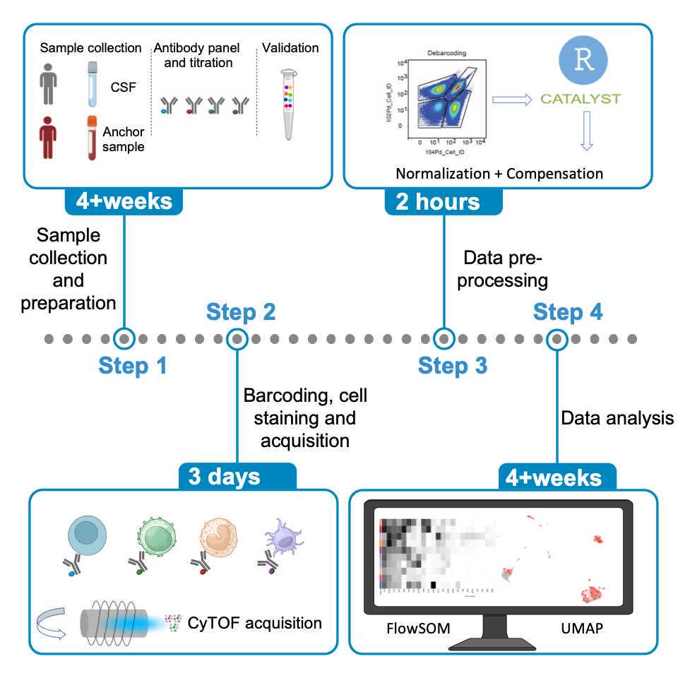
in CSF samples. Successful completion of the protocol (Figure 5) should enable the generation of different plots for data visualization using the CATALYST pipeline 15 .
Expected result
Figure 5. Workflow strategy to characterize immune cell populations by using CyTOF. Figure adapted with BioRender.com.
The Figure 4 present results from a small cohort of patients with CON (non-neuroinflammatory disease n=3), neuroinflammatory disease(n=4) and corresponding data analysis.
The MDS plot shows similarities between samples in unsupervised manner. On the other hand , the NRS plot identifies the ability of markers to explain the observed variance in each sample. Differences in cell compositions between CON and neuroinflammatory disease can be seen in the UMAP plots. To further evaluate the phenotypic differences of immune cells between the two conditions, we performed clustering analysis using the FlowSOM and ConsensusClusterPlus algorithms. A total of ten clusters were identified. Phenotypic differences in CSF B cells (Cluster 1) were detected between the two conditions. The proportion of CD19+ B cells was found higher in the neuroinflammatory patients than in the CON (Figure 4).
Before proceeding further with the analysis ,it is good practice to thoroughly examine the features of the dataset. As explained earlier in this protocol, it is important to consider which samples to include in the analysis. For instance, you may have outliers or a small number of cells in certain samples. In our analysis, we set a minimum of 10 cells per sample per cluster to consider for the clustering step. The individual operator must take this point into consideration, depending on the type of the dataset and the experiment they are working on.
Statistical analysis
30m
The method of our choice is edgeR test which is an optimal statistical test tool for low number of cells.
edgeR is a Bioconductor package for differential expression analyses. The package implements exact statistical methods for multigroup experiments developed by Robinson and Smyth. It also implements statistical methods based on generalized linear models (GLMs), suitable for multifactor experiments of any complexity.
# Create design matrix depending on your experiment
# Choose the features you want to test. In this example is selected condition_id
design < - createDesignMatrix(md, cols_design = "diagnosis_id")
# Create the contrast depending on the experiment and the objects chosen for the comparison (e.g ., CON vs MS)
contrast < - createContrast(c(0, 1))
#Perform the test
#Set the number for your "min_samples". Have a look at the number of your samples in the dataset. Min_samples refer to the smallest group between the two objects you are comparing.
res_DA_E < - diffcyt(sce, design =design, contrast = contrast,
analysis_type = "DA", method_DA = "diffcyt-DA-edgeR", clustering_to_use = "meta20", min_cells=3, min_samples=3)
# Show the p values
(top_DA_E < -topTable(res_DA_E, format_vals = TRUE, all=TRUE, show_counts = TRUE, show_props = TRUE))
Limitations
Sample staining and preparation for CyTOF can cause high rate of cell loss. Typically, only 50-70% of the sample can be recovered in the data. Therefore, studies involving rare cell populations require a larger starting sample size for adequate rigor as compared to studies investigating prevalent subset. The panel design is key to mass cytometry success. However, CyTOF experiments are still practically limited to around 60 markers, meaning that researches must still focus on particular types or functions of cells. Nevertheless, normalization methods and the use of anchor samples can be implemented to improve the reproducibility and comparability of CyTOF
results across experiments and study sites 1. Finally, the CSF studies usually fall short in providing longitudinal data because repetitive lumbar punctures are difficult to justify. Moreover, defining appropriate control groups is another crucial point because CSF samples from strictly healthy participants are usually not available6. However, together with the magnetic resonance imaging measures the CSF cell analysis can improve the diagnostic accuracy and help to estimate individual prognosis.
Troubleshooting
Problem 1 :
Due to the small number of cells, the generated pellet could be very small and difficult to see. ( before to begin)
Potential solution:
We recommended being careful during this passage and always double- checking the supernatant and the pellet. Leave a small amount of the supernatant with the pellet in the Falcon tube.
Problem 2 :
Contamination of CSF sample ( to begin). After centrifugation, the sample may contain blood droplets.
Potential solution :
Using a CSF blood-contaminated sample will affect the analysis and the reliability of the results. Therefore, we highly recommend excluding any contaminated samples from the analysis.
Protocol references
1. Fernández-Zapata, Giacomello, Spruth, Middeldorp, Gallaccio, Dehlinger ,Dames,Julia K. H. Leman, E. van Dijk, Meisel, Kunkel, Hol, Paul, Priller, and Böttcher.(2022). Differential compartmentalization of myeloid cell phenotypes and responses towards the CNS in Alzheimer's disease. Nat Commun.13:7210. https://doi.org/10.1038/s41467-022-34719-2.
2. Fangda Leng and Paul Edison. (2021). Neuroinflammation and microglial activation in Alzheimer disease: where do we go from here? Nature Reviews Neurology. 17, 157–172. https://doi.org/10.1038/s41582-020-00435-y
3. Thygesen, Rossel Larsen and Finsen. (2019). Proteomic signatures of neuroinflammation in Alzheimer’s disease, multiple sclerosis, and ischemic stroke. Expert Review of Proteomics. https://doi.org/10.1080/14789450.2019.1633919
4. Wong-Guerra, Calfio, Maccioni RB and Rojo LE. (2023). Revisiting the neuroinflammation hypothesis in Alzheimer’s disease: a focus on the druggability of current targets. Front. Pharmacol. 14:1161850. doi: 10.3389/fphar.2023.1161850.
5. Attfield, Jensen, Kaufmann, Friese and Fugger. (2022). The immunology of multiple sclerosis.Nat Rev Immunol.(2022). 22,734-750. https://doi.org/10.1038/s41577-022-00718-z.
6. Alvermann, Hennig, Stüve, MD, Wiendl, and Stangel. Immunophenotyping of Cerebrospinal Fluid Cells In Multiple Sclerosis. (2014). JAMA Neurol. 71(7):905-912. doi:10.1001/jamaneurol.2014.395
7. Heming, Börsch, Wiendl, Hörste.(2022). High-dimensional investigation of the cerebrospinal fluid to explore and monitor CNS immune responses.Genome Med.14:94. doi: 10.1186/s13073-022-01097-9.
8. Böttcher,Schlickseiser,Sneeboer,Kunkel,Knop,Paza,Fidzinski,Kraus,Snijders,Kahn,Schulz, Mei,Psy,Hol,Siegmund,Glauben,Spruth,d.Witte and Priller.(2019). Human microglia regional heterogeneity and phenotypes determined by multiplexed single-cell mass cytometry. Nat Neurosci.22,78-90. 10.1038/s41593-018-0290-2
9. Böttcher, Fernández-Zapata, Schlickeiser,Kunkel, Schulz ,E. Mei , Weidinger ,Gieß ,Asseyer, Siegmund ,Paul,Ruprecht and Prille.(2019). Multi-parameter immune profiling of peripheral blood mononuclear cells by multiplexed single-cell mass cytometry in patients with early multiple sclerosis. Sci Rep. 9:19471. https://doi.org/10.1038/s41598-019-55852-x.
10. Thrash, Kleinsteuber, Hathaway, Nazzaro,Haas, Hodi and Severgnini.(2020). High-Throughput Mass Cytometry Staining for Immunophenotyping Clinical Samples. STAR Protocols. 1,100055. https://doi.org/10.1016/j.xpro.2020.100055.
11. Maxpar Antibody Labeling User guide. FLUIDIGM. (2021). Rev 17.
12. Schulz, Baumgart, Schulze, Urbicht, Grützkau and Mei. (2019). Stabilizing Antibody Cocktails for Mass Cytometry. Cytometry Part A. 95A: 910-916. https://doi.org/10.1002/cyto.a.23781
13. McGuire and Ashhurst.(2019).Mass Cytometry, Methods and Protocols. Springer Protocols. https://doi.org/10.1007/978-1-4939-9454-0
14. Schuyler, Jackson, Garcia-Perez, Baxter, Ogolla, Rochford, Ghosh, Rudra and Hsieh. (2019). Minimizing Batch Effects in Mass Cytometry Data.Front. Immunol. 10: 2367.doi: 10.3389/fimmu.2019.02367.
15. Nowicka, Krieg , Crowell ,Weber Hartmann , Guglietta ,Becher ,Levesque and Robinson.(2017). CyTOF workflow: differential discovery in high-throughput high-dimensional cytometry datasets. F1000Research.6: 748.https://doi.org/10.12688/f1000research.11622.
16. Chevrier, Crowell, Zanotelli, Engler, Robinson and Bodenmiller. (2018). Compensation of Signal Spillover in Suspension and Imaging Mass Cytometry. Cell Systems. 6, 1–9. https://doi.org/10.1016/j.cels.2018.02.010